Documentation for TrendMiner’s Experimental package
Warning
This package is experimental. The definitions in this package can be changed or removed in future releases.
Anomaly Detection
The
anomaly_detetection
subpackage offers a custom TrendMiner model for
multi-variate, point-wise anomaly detection. The model is trained on a data frame containing
measurements taken during normal operation of your
process. That is, you create a view in TrendMiner with
normal behaviour of the process for which you want to
build an anomaly detection model.
Note
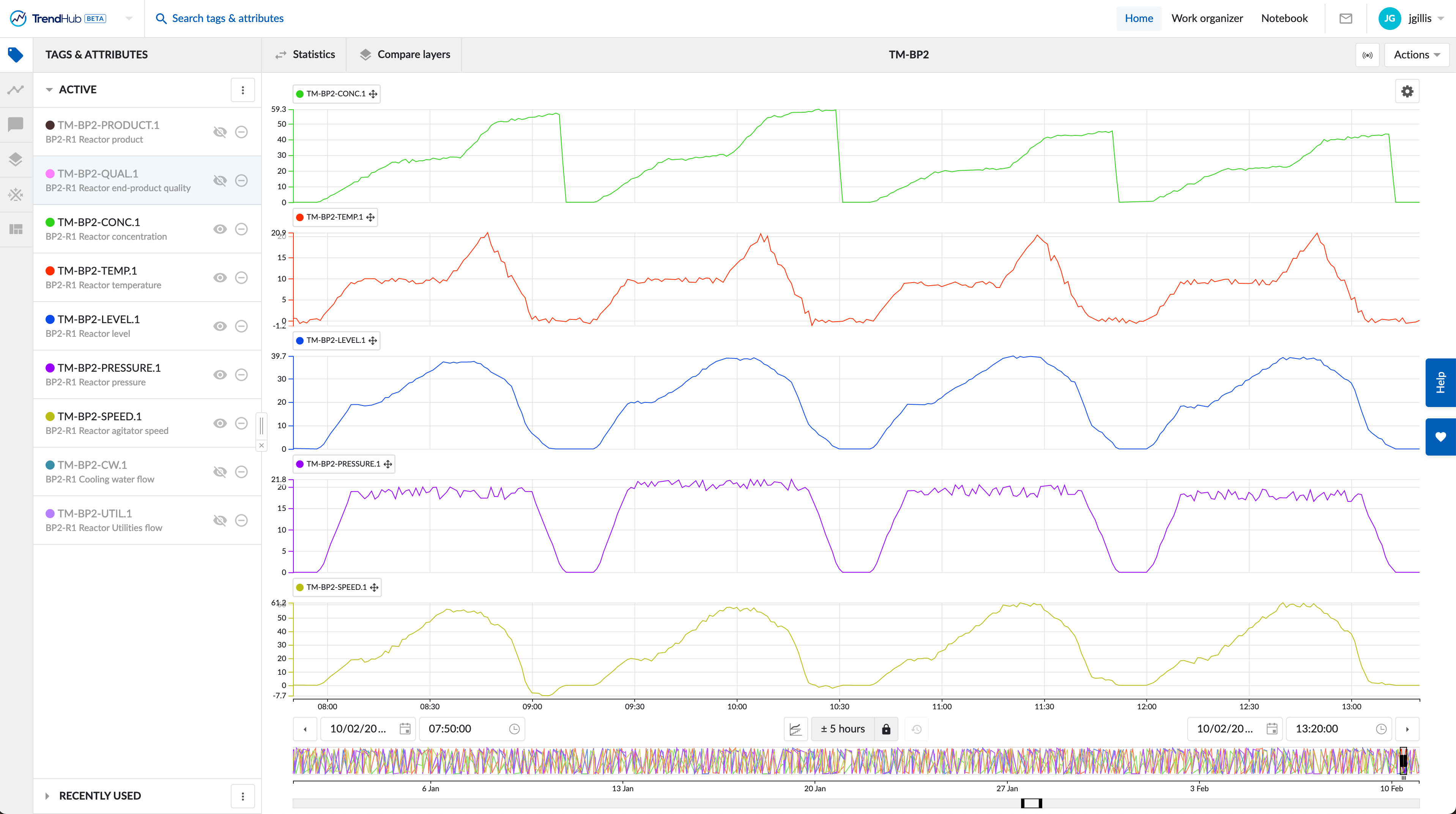
As an example flow for anomaly detection, you can load the TM-BP2 demo view from the tm-demo directory in work organizer. For this example, we will use the tags TM-BP2-CONC.1, TM-BP2-LEVEL.1, TM-BP2-TEMP.1, TM-BP2-PRESSURE.1 and TM-BP2-SPEED.1. This view consists of 6 hours of measurements representing normal operations. Typically, the more data that is in the view, the better the anomaly model will work.
The anomaly model is based on Self Organising Maps (SOM). Conceptually, the model fits a flexible two dimensional grid of units, on the training data set. Each unit can be though of as a n-dimensional cluster center, with n the number of tags in the provided view. In the training phase, the algorithm attempts to minimize the distance between the n-dimensional training data points and the nearest unit, whilst trying to keep the grid as smooth as possible to avoid overfitting on the training data.
Note
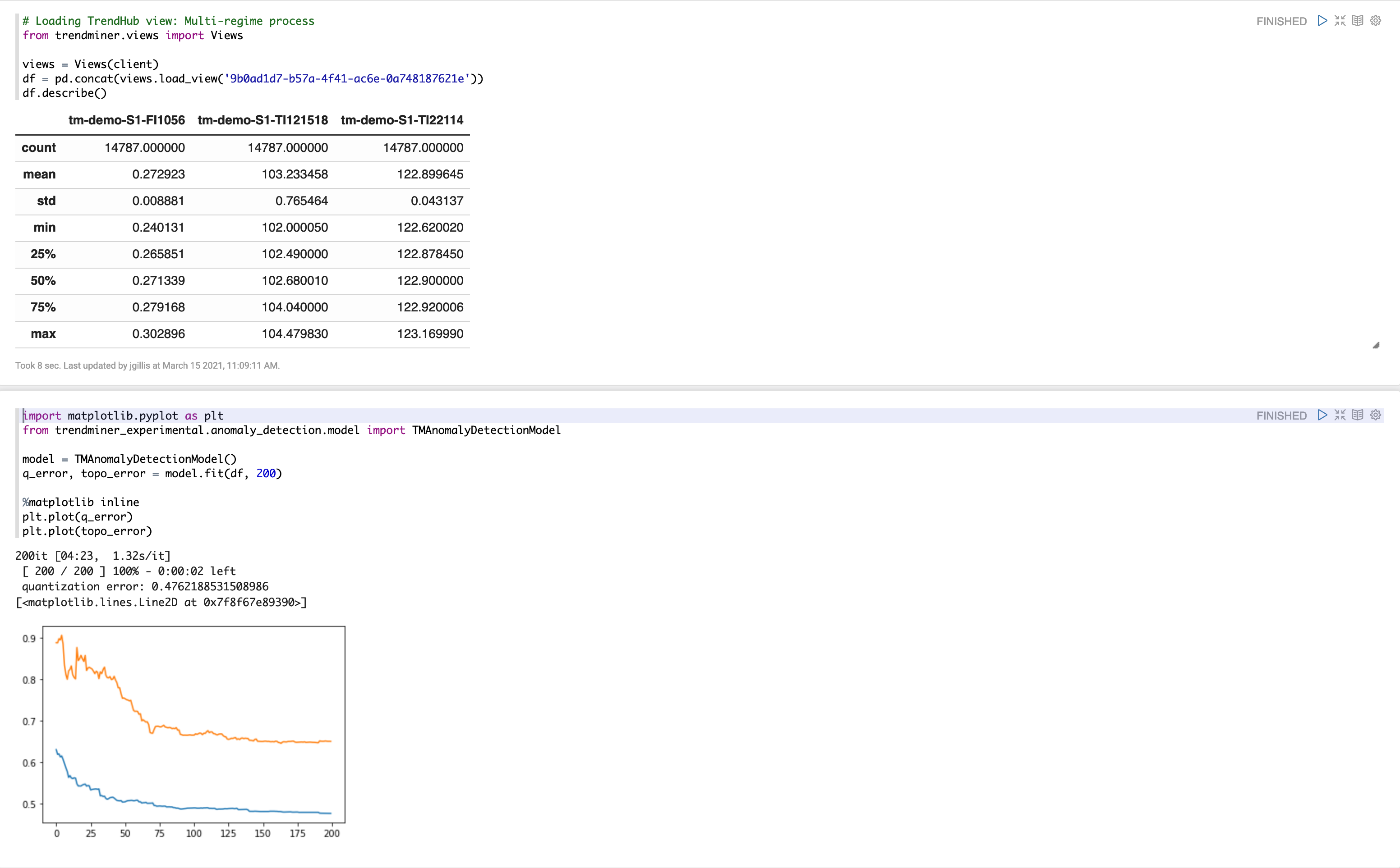
Open up a new notebook and load the TM-BP2 view into a data frame. Next, we import the anomaly model:
from trendminer_experimental.anomaly_detection.model import TMAnomalyModel

model = TMAnomalyModel()
q_error, topo_error = model.fit(df, 5000) # Training for 5000 iterations

import matplotlib.pyplot as plt
%matplotlib inline
plt.plot(q_error)
plt.plot(topo_error)
The fit method returns a list of quantization errors. This measures how far the training data points are from the units in the grid. A lower score indicates a better fit.
Once the model is trained on normal behaviour, we can
deploy the model on TrendMiner’s scoring engine. This
requires us to convert the model to its
PMML
form. The
TMAnomalyModel
has a utility method to convert the model to PMML:
to_pmml. This function takes two arguments:
-
The first argument is the name for the model. The name is used as the identifier of the model in the scoring engine. Ensure to choose a unique and descriptive name.
-
The second argument is the threshold percentage. It draws the line of what is considered an anomaly and what is normal. Typically, you want to set this to a high value, like 0.99, because we have trained on normal behaviour. Hence everything that is below the threshold according to the statistical distribution learned by the model, should be considered as not anomalous. On the other hand, everything above the threshold is considered anomalous. If you put the threshold percentage very high (above 0.99), beware that there are no outliers in your training data, because those points will be considered normal which could hamper the ability to detect anomalies.
Note
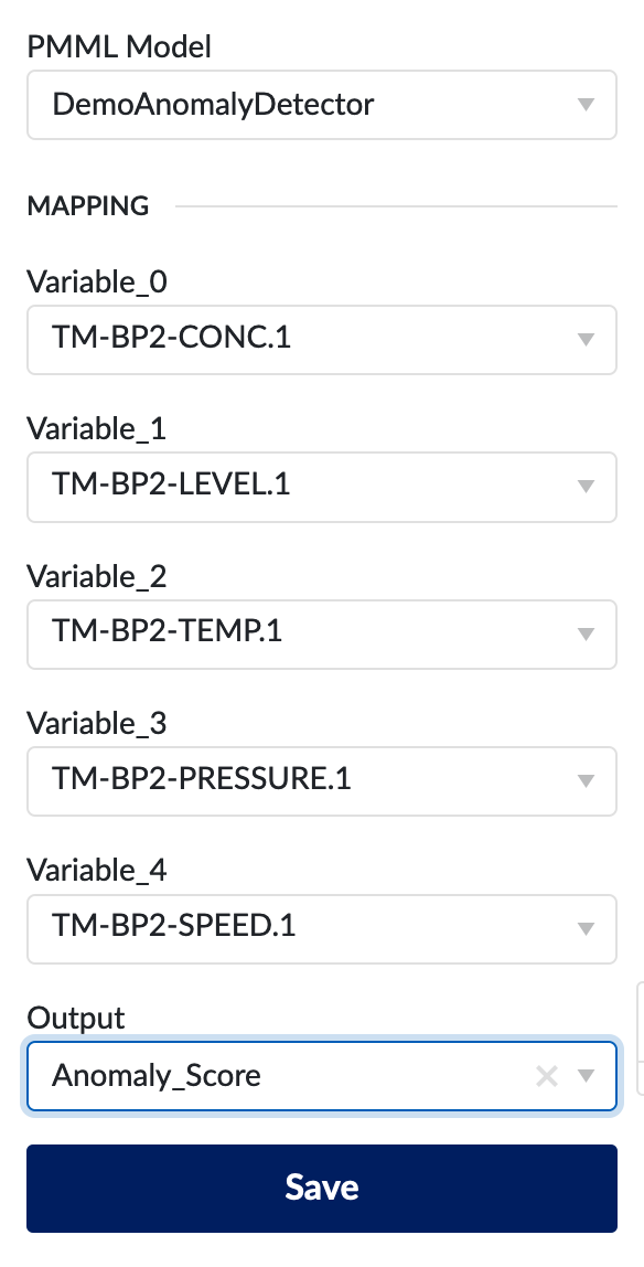
Finally, after training our model, we would like to use the model in TrendMiner. Open up the Machine Learning Model (MLM) option in the Tag Builder and select the model you just deploy to the internal scoring engine. Because we trained the model like this:
model = TMAnomalyModel()
selected_tags = ['TM-BP2-CONC.1', 'TM-BP2-LEVEL.1', 'TM-BP2-TEMP.1', 'TM-BP2-PRESSURE.1', 'TM-BP2-SPEED.1']
q_error, topo_error = model.fit(bp2_df[selected_tags], 5000)
there will be five variables to assign in the MLM menu.
Assign tags TM-BP2-CONC.1,
TM-BP2-LEVEL.1, TM-BP2-TEMP.1,
TM-BP2-PRESSURE.1 and
TM-BP2-SPEED.1 to the respective variables
in the model. Next, select
Anomaly_Score
as the output variable. A new time series with the
anomaly score at each point in time is created an
indexed in TrendMiner.
The
TMAnomalyModel
has two output variables:
Anomaly_Class
and
Anomaly_Score. The former,
Anomaly_Class, identifies a point as being anomalous or not, based on
the distance of the point to the closest unit in the model
and the threshold percentage you provided when converting
the model to its PMML representation. The latter,
Anomaly_Score, is the distance between a point and the closest unit in
the model.
Note
Once your MLM tag, based on the
TMAnomalyModel
with
Anomaly_Score
as output variable, is indexed, you can specify a VBS to
identify anomalies based on the score time series.
Enabling a monitor on this saved Value-Based search will
notify you when an anomalous period is detected.